The CoRsica Package for Hockey Analysis in R (0.1: Hello World)

EP: This is the second part in what I hope will become a lengthy and informative tutorial series on a pseudo-package I am building for R called coRsica. In this instalment, I’ll discuss the RStudio console and some R basics, and show you how to write your first script.

Inside RStudio
In section 0.0 you installed R and RStudio onto your computer. Now, I’ll quickly show you around the RStudio interface so you can make sense of it!

RStudio is an Integrated Development Environment, or IDE; but I prefer to simply call it a user interface for simplicity. What you should understand about it, regardless of your preferred terminology, is that RStudio offers a comprehensive environment for you to program in R. Using RStudio should make your life easier, particularly as a beginner, so it’s a valuable tool to familiarize yourself with. Pictured below is the RStudio interface divided into its major elements:

In this tutorial, I’ll refer to these four elements as follows:

1. The Text Editor
2. The Console
3. The Workspace
4. The Viewer

You may see them named differently elsewhere, but these are simply my conventions.

The Text Editor
If you are currently looking at your RStudio interface for the first (or second, if you took a peek after installing) time, you may not see this section just yet. Don’t worry – that just means you haven’t started to write scripts yet. As the name implies, this is your text editor. It is set to recognize R code and will colour-coordinate certain elements, promote consistent indentation and do all sorts of other cool things depending on the version you’re using. It’s probably best to give yourself some time to experiment before you begin worrying about the idiosyncrasies of the text editor. As you’ll find, it’s quite intuitive and easy to use.

This is where you will write .R files – scripts. These are blocks of R code that are stored in files that can be edited, deleted or executed at your convenience. Scripts will make more sense as you begin to learn what R code can do, and by the end of this section you will have written your very first program.

The Console
The console is where you can submit R commands and view output. When you boot up RStudio, the console will have printed out some basic information about the version you’re using and ways to ask for various details. The single-quoted words followed by closed brackets (ex: ‘help()’) are your first taste of functions, a concept I’ll discuss in greater detail later on. The > symbol is prompting you for input, so let’s enter our first command! Start with something simple, like addition. Follow my syntax below, but feel free to substitute the numbers with your own. Use the + operator between your numbers and press enter to submit your code:

> 2 + 6
[1] 8

Note that we supplied input, and received an output. By default, the vast majority of R commands will return a value. Here, the result of the mathematical expression you submitted was printed out in the console (ignore the [1] for now).

The value returned by a command will be printed out this way unless you assign it to an object. Objects are variables of all shapes and sizes that can store data. You can give an object any name you wish within the accepted nomenclature¹”A syntactically valid name consists of letters, numbers and the dot or underline characters and starts with a letter or the dot not followed by a number. Names such as ‘.2way’ are not valid, and neither are the reserved words.” https://stat.ethz.ch/R-manual/R-devel/library/base/html/make.names.html , and the <- symbol or = sign can be used interchangeably to do so. To segue into the next section, go ahead and assign a number between 1 and 10 to the variable y as I’ve done below:

> y <- 3

As a final exercise, enter the three following commands into your console:

> “corsica”
[1] “corsica”
> corsica
Error: object ‘corsica’ not found
> #corsica

Did the final command do anything? You’ll find out later.

The Workspace
You’ll notice that the workspace area of your RStudio environment is no longer empty. This means that you’ve successfully populated it with your first object. The workspace lists and displays information about objects in the R environment. Every time you create a new object, it’s added to the workspace. In the upper-right corner of this area, you should see the word “List.” This option controls how objects are displayed in your workspace. My preference is to use the “Grid” option, as it allows me to clear selected objects more easily. Go ahead and switch to the grid view (you can switch back according to your own preference later):

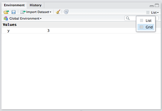
You should now see additional details about the variable y you created. It’s not important that you understand what it all means at this point, though you can probably guess.

The broom icon on the toolbar is used to clear, or delete, objects from the workspace. As I mentioned before, the grid view lets you select which objects to clear by checking the boxes to the left. By default, clearing the workspace will delete all objects.

The familiar disk icon to the left can be used to save your workspace as an .RData file. This is a lightweight file type that will store information about your R sessions. When you load an .RData file, which you’ll learn to do later on, RStudio will import all the stored objects into your current session.

The Viewer
I won’t spend too much time on this because I typically only use the viewer to view plots I’ve generated, but there are other uses worth knowing about. The viewer is a multi-purpose area of your RStudio interface used to display relevant information. As I mentioned, this is where plots are shown. You can also use the viewer as a file manager, by selecting the Files tab. It can also display documentation on various R functions under the Help tab. To ask for help, lead a particular function name with a question mark. Ask about the print() function by entering the command below:

> ?print

Feel free to read the documentation as we’ll be using this function shortly.

Hello World
You’re almost ready to write your first R script. There’s just a little more you should learn about objects, classes and comments. Recall the exercise at the end of the Console section. Why is it that the unquoted command returned an error while the “corsica” command did not? The reason is that when given text that is not between quotation marks, R will look for an object or function of that name. Since corsica is neither, the console returned an error (and a descriptive one). Try instead to specify an object you know exists, because you created it:

> y
[1] 3

Because we stored a value in the object y, we can call it as a variable to return that same value whenever we want. To see how this works, use the – operator to subtract 1 from y:

> y – 1
[1] 2

Now, what if we wanted to store the result of y – 1 to a new variable x? You should be able to guess by now how this works:

> x = y – 1
> x
[1] 2

Note how I used the = sign rather than the <- symbol to assign a value to x. This is simply to show that both are equivalent, though I prefer <- and will stick to that going forward. Try multiplying y by x using the * operator.

> y * x
[1] 6

So what happens when you try to call y between quotations? Does RStudio print out the value stored in y like before (it shouldn’t)? This is because quotation marks specify that you are creating a string, which is just a fancy word for a collection of characters. You can use single or double quotes, but can’t close one with the other (ex: ‘corsica” or “corsica’). Let’s create a new object called my_name and assign to it the value of a string containing your name:

> my_name <- “Emmanuel”
> my_name
[1] “Emmanuel”

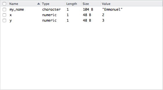
We’ve just shown that values in R are not limited to numbers. Indeed, there are a variety of different object classes that store different types of data. If you are using the grid view in your workspace, you should see the distinction under the “type” header:

The last lesson before finally writing our first script is comments. These are not a class, but a syntax rule in R. Recall that entering #corsica into the console did not return a value or seemingly do anything. That’s because in R code, anything to the right of a pound sign is inert. We call these comments or annotations. Because comments will not be rendered as R code, we can use them to safely write notes in our scripts. It’s good practice to annotate one’s code, for the benefit of others if not your own. In the future, I’ll use comments in the example code which you do not need to transcribe.

> “Corsica”        # This is a string
[1] “Corsica”     # This is output

What you’ve learned so far may not seem like much, but it’s enough for you to write your first script. Go ahead and open a new file in the text editor if you haven’t already.

You can save a file even though it’s empty, so use the disk icon at the top-left to save the blank script as hello.R. I always think it’s better to form good habits early on, so let’s use comments to write some information about the script at the very top:

# Hello World
# Last edited on 08-14-2016

For those unfamiliar with programming, Hello World is a common first exercise used to introduce users to the language’s syntax. The purpose is simply to display “Hello, world!”. Sounds easy enough, right?

If your viewer no longer shows the documentation for the print() function, go ahead and ask the console again using the question mark. It’s not necessary to understand everything about this function just yet. The important takeaway is that the print() function takes an argument and, as the name implies, prints it out. We’ll use this function to print the words “Hello, world!”, but first, we’ll use our knowledge of objects to store the desired string. On line 5 of your script, store the value “Hello, world!” in the object my_string:

# Hello World
# Last edited on 08-14-2016

my_string <- “Hello, world!”

Use the line 4 to write a comment explaining the next step of the script. Note the blank line separating the topmost comments and the next “section” of the script. This is my convention, as I think it makes things tidier.

Now that you’ve stored your string in a variable, you can use the print() function to display it. As explained in the documentation, print() is designed to be able to handle arguments of various classes. Here, we’re supplying a character, which is easily processed. Add the following code to line 8, with a comment on the line above it:

print(my_string)

Your script is now functional and ready for testing. To run the code in your text editor, first select the code you wish to execute. You may triple-click to select entire lines (though, by default RStudio will run the line your cursor is currently on) or quadruple click to select the entire file (Command+a also works). The Run icon at the top-right of the text editor will execute the selected code, or you can use the keyboard shortcut Command+Enter. Save your hello.R file, then use your preferred method to run the entirety of it.

[1] “Hello, world!”

Congrats! You just wrote and executed your first R script. If your console did not print out the above output, copy the code below and try again:

EP: It was brought to my attention that the formatting of the text below does not agree with the RStudio text editor. Please transcribe the code instead of pasting.

# Hello World
# Last edited on 08-14-2016

# Store string in object
my_string <- “Hello, world!”

# Print string
print(my_string)

When you’ve successfully printed out “Hello, world!”, edit your code to resemble mine below²The colour scheme I use is a matter of preference. You can choose your own by following RStudio > Preferences > Appearance from the top menu. :

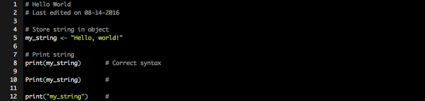
Complete the comments on lines 10 and 12 with what you think is wrong with the print syntax on that line. Once you’ve done that, run the entire script.

> print(my_string)         # Correct syntax
[1] “Hello, world!”
>
> Print(my_string)         # print() should not be capitalized
Error: could not find function “Print”
>
> print(“my_string”)     # my_string should not be quoted
[1] “my_string”

The error message obtained from the second command shows that R is case-sensitive. This is an important feature, as it means print() and Print() are not syntactically equivalent. The third command did not produce an error, though it did not achieve what we wanted, either. By putting my_string between quotations, you’re telling R that it’s a character whose value is equal to “my_string.” Hence, the value “my_string” is passed as an argument to print() instead of the value stored in my_string. Remove the faulty code and save hello.R as we’ll use it later.

In the next section, we’ll go over some fundamentals of R to build the foundation for a deeper understanding of the language.