
EP: This is the 1.5th instalment of the Shot Quality and Expected Goals series. Read the first part here.
I finished the first part of this series with a promise of certain things to follow in the next. Those things were delayed and eventually superseded by a pressing request I’ve heard echoed since the launch of the site. When WAR On Ice closed its doors, implementing scoring chance data became a top priority.
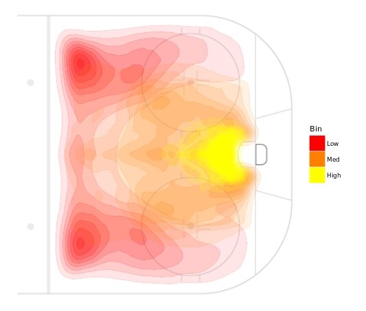
WAR On Ice employed the idea of zones to attribute shot quality. By assigning an expected goal likelihood to shots originating from various bounded spaces on the ice surface, they arrived at three danger tiers: High, medium and low danger. In reality, this method involved other considerations such as blocked, rebound and rush shots, but the principle of spatial classification remains. The use of danger zones yielded two scoring chance definitions (regular and high-danger) and new possibilities when it came to evaluating goaltenders. In particular, how do goalies perform against shots from each zone and how was their total performance after accounting for the nature of each shot faced?
In addressing these features, I chose to do things a little differently. I opt to employ the existing shot quality model used throughout the site in place of simple shot location. That is, rather than categorize shots by their location, I categorize them based on their estimated xG value. I believe this adds a level of sophistication to the approach in addition to solving a fundamental flaw in the xG model, as I’ll show later on.
The danger zone1Henceforth, “danger zones” should be understood to be figurative and interchangeable with “danger tiers.” definitions are responsibly arbitrary. Let me explain. In absence of a universally decreed rule, I look only to satisfy certain requirements. I make no claim that this set of danger zones is true or correct because I don’t believe there is such a thing. However, I acknowledge the responsibility to produce something that makes sense, and that has value. To clarify that “arbitrary” is not a dirty word in this sense, consider the home plate scoring chance area:

This construct would not exist in a parallel world where hockey was played on a blank ice surface. Shots from this area are far more likely on average to result in goals, yes. But the exact boundaries are a product of visual reference points. Consider an alternate home plate area – one that extends an additional five feet beyond the line drawn between the top of the circles. It is reasonable to expect that this is also an adequate scoring chance area. The sacrifice we make here is one of convenience, not necessarily accuracy.
With this in mind, I impose the following rules for a satisfactory set of xG-delimited danger zones:
- The true shot quality of each zone should reflect the low-medium-high convention.
- The mean shooting percentage of medium-danger shots should be approximately equal to the league average shooting percentage.
- Each zone should contain a sufficient fraction of total shots.
- The xG bins forming each danger zone should be easy to remember.
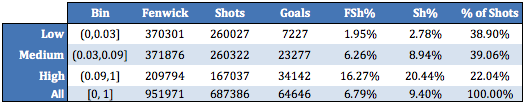
The bins I settled on are as follows:
Low Danger: less than 3.0%
Medium Danger: Less than 9.0% and equal or greater than 3.0%
High Danger: Equal or greater than 9.0%
To avoid confusion, I’ll offer this reminder: xG is based on unblocked shots. As such, it is interpretable as Fenwick Shooting Percentage. When discussing LD/MD/HD shots on goal, we’re talking about shots on target whose estimated Fenwick Shooting Percentage belonged to the respective range detailed above. Hence why the mean Medium-Danger Sh% is roughly league average (~9%).
A benefit of this method is we’ve developed an implicit conversion from xG to Sh%. Granted, it is oversimplified. Nevertheless, we can assume with varying confidence that a number of shots belonging to a danger tier will resolve to a certain mean shooting percentage. We observe how this confidence interval shrinks as our sample size increases:
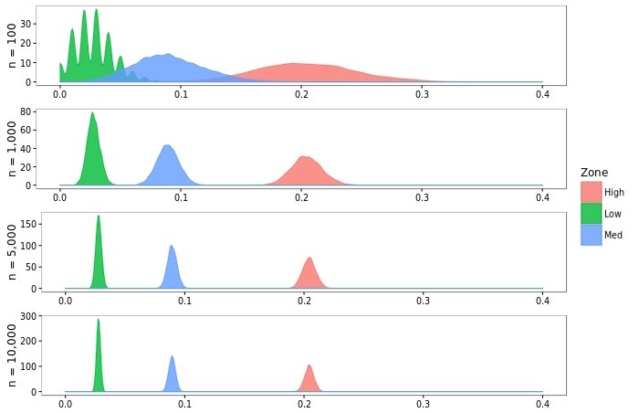
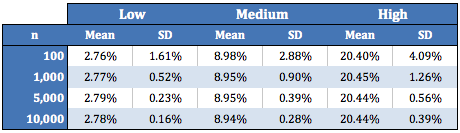
The following table summarizes the distributions obtained from selecting 5,000 random samples of n shots belonging to each danger zone:
We may use these standards to develop an expectation for goals allowed based on the shots faced by a goaltender. There is no value in comparing save percentage with the total shot quality faced as described by xG because it represents Fenwick Shooting Percentage. Hence why Adj. FSv% is included in the goalie stats while Adj. Sv% is not. We can, however, use the estimate of goals allowed based on danger zones to measure performance. Let GSAA (Goals Saved Above Average) be equal to the net difference between the number of goals allowed by a goaltender and the quantity expected from the danger of shots faced.
GSAA = (0.0278*LDSA + 0.0894*MDSA + 0.2044*HDSA) – GA ,
where LDSA, MDSA and HDSA are Low-Danger, Medium-Danger and High-Danger shots against, respectively, and GA is the number of goals against. As a preliminary test of validity, we can confirm GSAA persists reasonably well across seasons; as does GSAA/30, Goals Saved Above Average per 30 shots:
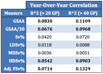
Additionally, it appears the skill-driven component of Sv% is almost entirely contained in a goalie’s ability to stop shots of the High-Danger variety.
Danger zones offer a convenient method of defining scoring chances. The legwork of determining shot quality has already been done by the xG model and our High-Danger tier is more than suitable to describe scoring chances. As shown above, the mean FSv% of High-Danger shots is 16.27% and the mean Sh% is 20.44%. Scoring chances may be defined as unblocked shots belonging to the High-Danger zone – that is, whose xG is equal to or exceeds 0.09. For convenience, one can approximate that one goal is scored for each 6 scoring chances. My personal preference is to use xG over scoring chances as it represents a continuous shot quality scale, but I appreciate that scoring chances are easier to digest for most.
My intention for part 2 of this series is still to offer practical applications of xG, which now includes danger zones and scoring chances. Namely, how and when we can use the information supplied by the xG model to inform better predictions than are offered by common alternatives.
References
| 1. | ↑ | Henceforth, “danger zones” should be understood to be figurative and interchangeable with “danger tiers.” |